A project finance model is easier to review when you can follow the calculations from the assumptions to the returns. That sounds obvious, but it is surprisingly easy to lose that thread once a template has been adapted for a particular deal.
This article walks through an example workbook, sheet by sheet. The project is an imaginary wind farm with 80 turbines. Construction takes eight quarters from January 2027, operations run for ten years from 2029, and construction costs are about $332m including a 10% contingency.
All figures are illustrative and were invented for teaching. The useful part is the model structure, not the investment case.
How the sheets fit together
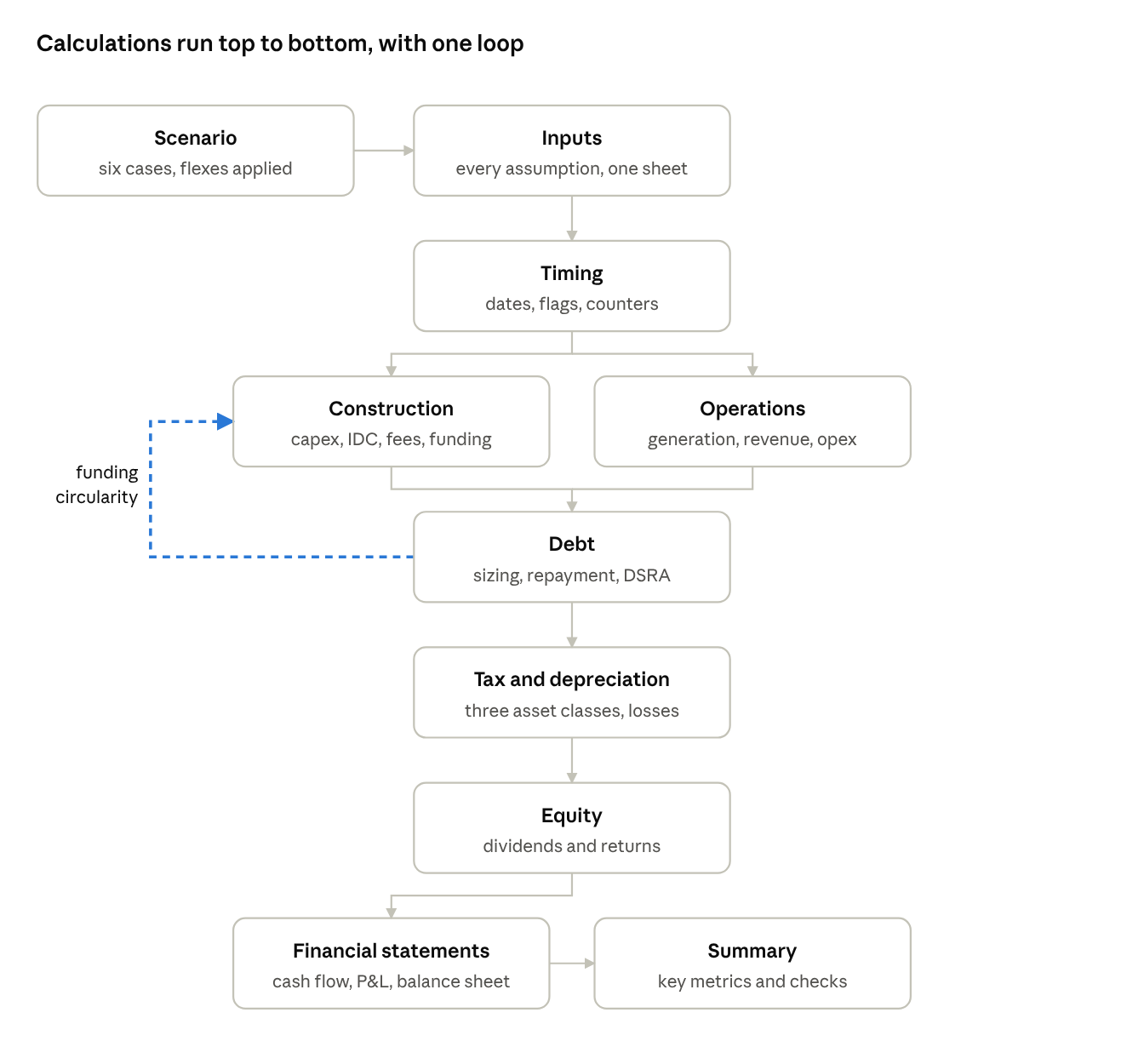
The calculations generally run in one direction. The Scenario sheet selects the case and applies its adjustments. Inputs feed Timing. Timing feeds Construction and Operations, which feed Debt, then Tax and Depreciation, then Equity. The results come together in the integrated financial statements and Summary.
Each calculation sheet starts with the same twelve rows: period dates, construction and operations flags, counters, and days in the period. A sheet called Copy holds the master layout so those headers remain consistent.
The columns are quarterly and line up across the workbook. Column R represents the same quarter on Operations as it does on Debt. Keeping that alignment makes formulas easier to trace and reduces the chance of linking to the wrong period.
The funding calculation is the main exception to the one way flow. It is circular, so it needs a separate, controlled process.
Inputs and cell styles
All assumptions sit on one Inputs sheet. A style legend distinguishes assumptions, technical inputs, links within a sheet, links from other sheets, subtotals, totals, flags and closing balances. A reviewer should be able to identify an input without inspecting its formula.
The cost tables also include spare rows. Adding a cost line late in a transaction is common. Having room for it is safer than inserting rows into a working model and hoping every range adjusts correctly.
The main operating assumptions are:
- 80 turbines producing 12,500 MWh each per year.
- Overall efficiency of 97%.
- A base electricity price of $112/MWh, with high and low price inputs of $155/MWh and $105/MWh.
- About $5m of annual fixed operating costs, escalating at 2.2%.
- Variable operating costs of $1.30/MWh and a tax rate of 30%.
Timing flags
The Timing sheet turns the project dates into construction and operations flags, operating year counters and a cost escalation index. Those flags control when calculations are active.
For example, revenue is generation multiplied by price and the operations flag. It does not need a separate nested IF statement for each period or a hardcoded start column.
If the technical adviser moves the commercial operation date (COD) by a quarter, changing that date should move the relevant calculations throughout the workbook.
Construction and funding circularity
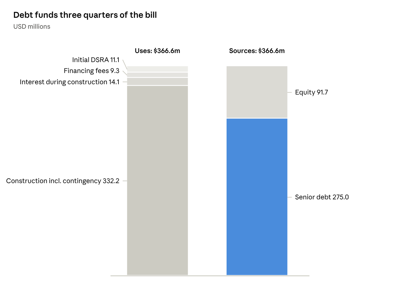
Total uses of funds are $366.6m, covering construction, interest during construction (IDC), financing fees and the initial debt service reserve account (DSRA). The funding split is 75% senior debt and 25% equity.
| Item | USD millions |
|---|---|
| Construction including contingency | 332.2 |
| Interest during construction | 14.1 |
| Financing fees | 9.3 |
| Initial DSRA | 11.1 |
| Total uses | 366.6 |
| Senior debt | 275.0 |
| Equity | 91.7 |
| Total sources | 366.6 |
Figures are rounded individually, so the displayed components may not add exactly to the totals.
The circularity comes from interest and fees. Both depend on the size of the loan, but the size of the loan depends on total uses, which include that interest and those fees.
This workbook resolves the loop using copy and paste macros. Each circular item has a Copy, Paste and Delta range. The macro copies the calculated result and pastes it as a value until the delta reaches zero. The DSRA target and loan life cover ratio (LLCR) sizing use the same approach.
A closed form solution may be possible in a simpler model. Here, the separate ranges make the process visible to a reviewer, and Excel's iterative calculation remains switched off. Whichever method is used, convergence alone is not proof that the model is correct; the result still needs to be checked.
Operations
Annual generation is 80 turbines multiplied by 12,500 MWh and 97% efficiency, giving 970,000 MWh, or 970 GWh. At $112/MWh, annual revenue is about $108.6m.
Fixed operating costs are entered in real terms and escalated. Variable costs follow generation at $1.30/MWh.
The workbook also includes working capital, with 30 debtor days and 60 creditor days, and interest on cash balances. These items have a relatively small effect on returns in this example, but omitting them would leave the cash flow and balance sheet incomplete.
Debt sizing and repayment
The debt amount is the lower of two limits. The 75% gearing cap allows $275.0m. An LLCR target of 2.0x at COD would allow $283.7m.
Gearing therefore limits the loan in the base case. The cash flows could support about $9m more debt under the LLCR test if lenders were willing to relax the gearing cap. That is useful information when discussing the term sheet.
Repayment can be calculated as an annuity or sculpted to a target debt service cover ratio (DSCR), set here at 1.25x. The interest margin falls from 3.2% during construction to 1.9% by year four. The upfront fee is 1%, and the commitment fee is half the margin on undrawn amounts.
The base case produces a minimum DSCR of 1.98x and an LLCR of 2.03x.
The cash flow waterfall
The waterfall sets the order in which project cash is used. Shareholders receive distributions only after the obligations above them have been met.
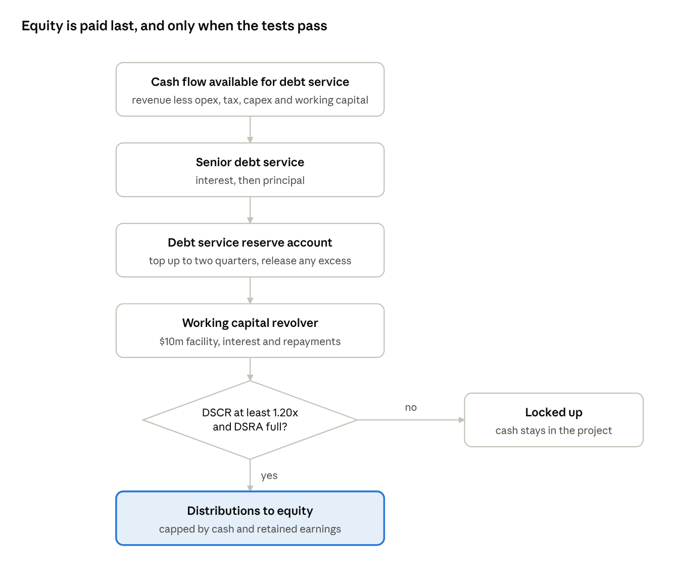
- Cash flow available for debt service is calculated after operating costs, tax, capital expenditure and working capital movements.
- Senior debt interest and principal are paid.
- The DSRA is maintained at its target of two quarters of debt service. It can cover a shortfall, receive a top up or release excess funds as the target falls.
- The $10m working capital revolver is serviced, including interest and repayments.
- Distributions are tested against the 1.20x DSCR lock up threshold and the requirement for a fully funded DSRA.
- Any permitted distribution is capped by available cash and retained earnings. If the tests fail, cash stays in the project.
Tax, depreciation and the dividend trap
Assets are grouped into three classes: long term assets, short term assets and capitalised financing costs. Accounting depreciation is straight line, tax depreciation uses a reducing balance method, and tax losses carry forward.
A separate unlevered tax calculation feeds the project internal rate of return (IRR). This keeps the project return separate from the benefit of the interest tax shield.
In this example, dividends are capped at the lower of available cash and retained earnings. Accounting profit can lag cash generation in the early years, leaving cash in the project that cannot yet be distributed under that rule. This is often called the dividend trap. Actual distribution restrictions depend on the applicable law and financing documents.
Checks on every sheet
The integrated financial statements contain the cash flow waterfall, income statement and balance sheet. Two balance sheet checks feed a master integrity flag. Warnings, such as an underfunded DSRA, feed a separate master signal. The macro deltas provide a third check.
All three are shown at the top of every sheet. An unresolved check should be investigated before the model is circulated. A balancing balance sheet is necessary, but it does not replace a review of the assumptions and formulas.
What the scenarios show
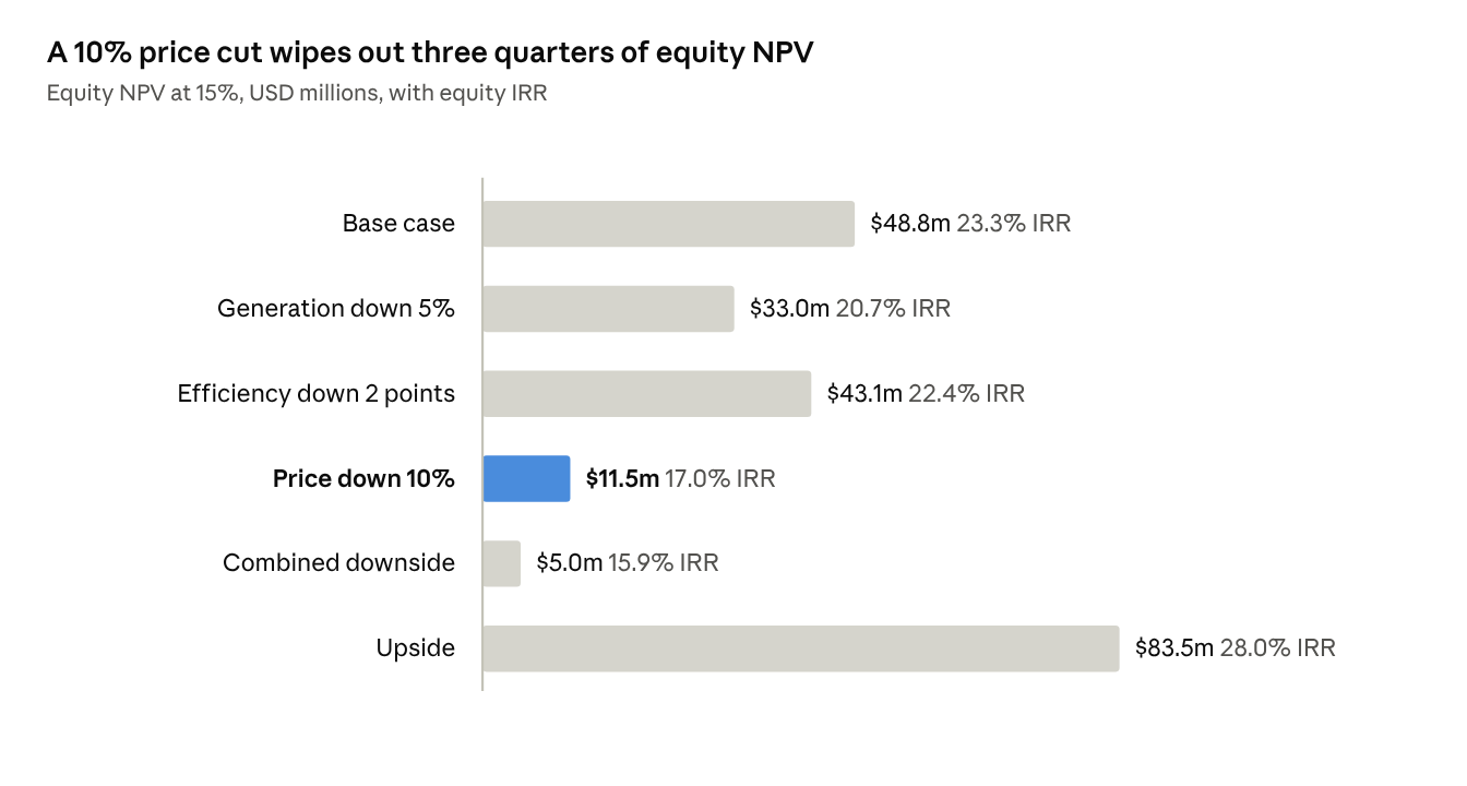
The base case produces a project IRR of 20.3% and an equity IRR of 23.3%. A macro runs six scenarios and records the results.
| Scenario | Equity NPV | Equity IRR |
|---|---|---|
| Base case | $48.8m | 23.3% |
| Generation down 5% | $33.0m | 20.7% |
| Efficiency down 2 percentage points | $43.1m | 22.4% |
| Price down 10% | $11.5m | 17.0% |
| Combined downside | $5.0m | 15.9% |
| Upside | $83.5m | 28.0% |
A 10% reduction in the electricity price takes equity net present value (NPV) from $48.8m to $11.5m, a fall of about 76%. A 5% reduction in generation reduces NPV by $15.8m. A two percentage point reduction in efficiency reduces it by $5.7m.
Price is the largest of those individual risks in this example. The model gives a practical reason to spend time on the power purchase agreement (PPA): a relatively modest change in the contracted price has a much larger effect on shareholder value.